SVDQuant: Absorbing Weight Outliers into a Low-Rank Branch for 4-Bit Diffusion Models

Notes on SVDQuant (ICLR’25 Spotlight), a W4A4 post-training quantization method for diffusion models. The core idea: activation smoothing alone doesn’t remove quantization difficulty, it just moves it from activations to weights — so SVDQuant follows up by decomposing the smoothed weight into a low-rank outlier branch (kept in higher precision) and a residual (quantized to 4-bit), then fuses the two branches into a single kernel to keep the low-rank branch from adding latency. (ref: video walkthrough)

01. Introduction

A. Related Works

Symmetric quantization only requires a scaling factor, while asymmetric quantization also requires a zero point (shift). Symmetric is more widely used because it has less overhead.

a. SmoothQuant (ICML’23)

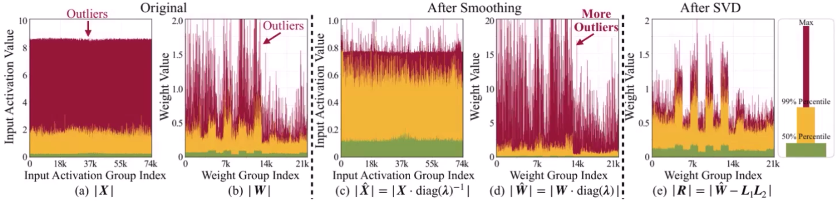
Activations are harder to quantize than weights, mainly because of outlier channels. SmoothQuant addresses this by migrating quantization difficulty from activations to weights via a per-channel smoothing factor — it assumes that weight quantization “would not become harder after smoothing.”

In reality, though, quantization difficulty is transferred from activations to weights after smoothing, not eliminated. There is follow-up research addressing this transferred difficulty directly, using iterative or learnable approaches. SVDQuant is one of them.

Figure 1. Smoothing moves outlier magnitude from activations into weights — it doesn't remove it.

b. QLoRA (NeurIPS’23)

Inspired by the LoRA architecture, SVDQuant builds a low-rank branch ($L$) to absorb outliers, following a mixed-precision approach.

SVDQuant’s architecture resembles QLoRA’s — quantizing only the pre-trained weights while keeping an adapter branch in full precision. But QLoRA was designed for fine-tuning, not inference; its low-rank branch is a dense, unfused nn.Linear add-on, which is exactly the part that’s hard to accelerate at inference time. SVDQuant instead fuses that branch into its kernel (§02.D) so it doesn’t cost extra latency.

02. Method

A. Quantization Error Decomposition

Quantization is an optimization problem: minimize accuracy error and memory footprint while maximizing throughput.

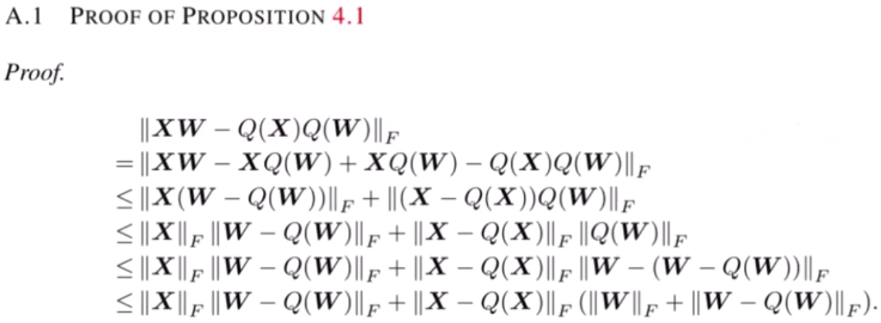
Quantization error is the distance between the full-precision model and the quantized one — i.e., between the outputs of the original and quantized layers:

\[Error \approxeq E(X, W) = \|XW - Q(X)Q(W)\|_F\]

This error is bounded by four terms — $

W

$, $

X

$, and their respective quantization errors $

W - Q(W)

$, $

X - Q(X)

$ — derived purely via the triangular inequality. SVDQuant’s whole design targets these four terms.

Figure 2. Quantization error decomposition via the triangular inequality.

B. LoRA Architecture

After activation smoothing, quantization difficulty now sits in the weights rather than the activations (§01.A). So SVDQuant decomposes the smoothed weight $\hat{W}$ into two low-rank branches $L_1, L_2$ and a residual $R$: $L_1 L_2$ captures the outliers in the weight, and $R$ contains only the non-outlier values.

Figure 3. Weight decomposition into a low-rank outlier branch and a quantization-friendly residual.

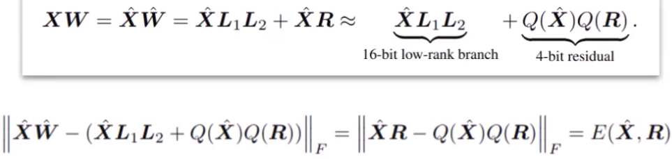
By this construction, $R = \hat{W} - L_1 L_2$, so $

R

_F$ is minimized by choosing $L_1, L_2$ optimally. Finding that optimum is where SVD comes in.

C. Singular Value Decomposition (SVD)

The goal: find $L_1, L_2$ that minimize $

R

_F =

\hat{W} - L_1 L_2

_F$. The authors solve this via the Eckart–Young–Mirsky theorem — $\hat{W}$ can be decomposed via a single SVD, and truncating to rank $r$ (keeping only the top-$r$ singular values/vectors) gives the optimal rank-$r$ approximation, minimizing the residual in Frobenius norm.

By SVD, the largest singular values (outliers) are selected into $L_1 \cdot L_2$, leaving the residual $R$ free of the values that were hardest to quantize.

Note: The paper doesn’t elaborate on how $L_1, L_2$ are actually computed at rank-selection time. Left as a TODO to fill in after reading the deepcompressor source.

D. Nunchaku Kernel

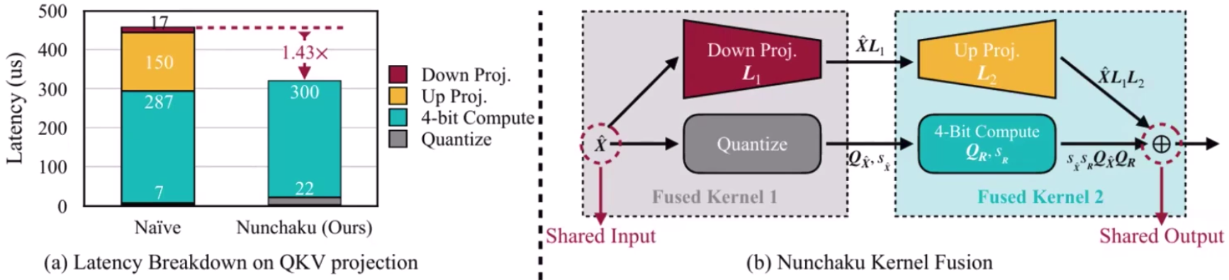
Splitting the weight into two branches only pays off if the low-rank branch doesn’t add its own latency tax. SVDQuant’s Nunchaku kernel is designed specifically to remove that tax:

• The Down-Projection and Quantize kernels consume the same input, and the Up-Projection and 4-bit Compute kernels produce the same output.
• To cut data-movement overhead, SVDQuant fuses the first pair and the second pair together, rather than launching them as four separate kernels.

Figure 4. Nunchaku fuses the low-rank branch's projections with the residual branch's quantize/compute stages.

03. Personal Comments

SVDQuant, also known as a Nunchaku, is a mixed-precision technique for diffusion model w4a4 (quantize both weight and activation to 4-bit) inference. It follows low-rank decomposition to extract outliers and quantization error, and it’s formula is easy to understand. Fused kernels are published to Nunchaku, and maintainers have been continuously expanded support to variable model series like Qwen-Image and Tongyi-MAI/Z-Image-Turbo.

---

References

• SVDQuant (ICLR’25 Spotlight): video walkthrough
• SmoothQuant (ICML’23): Accurate and Efficient Post-Training Quantization for Large Language Models
• QLoRA (NeurIPS’23): Efficient Finetuning of Quantized LLMs
• Nunchaku / deepcompressor: https://github.com/namgyu-youn/deepcompressor/tree/main/deepcompressor